Making a LookUp Table, stops after reaching first occurrence of Keyword

[TinySpoon]

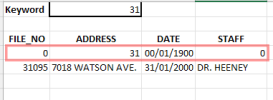
I'm trying to create a lookup formula searches a table for a keyword, then returns the entire row when a keyword match is found anywhere within that row.
Most importantly, it needs to return every row with that keyword. It also needs to return partial keyword matches and not case sensitive. Lastly, the keyword could be a number or text.
The table is populated with numbers, names, addresses, and dates.

Example:

FILE_NO	ADDRESS	DATE	STAFF
10450	51 st & CLARK	01/01/2000	DR. WATSON
180093	1300 S. MAIN ST.	01/18/2000	DR. WATSON
31095	7018 WATSON AVE.	01/31/2000	DR. HEENEY
9000078	5010 WATSON AVE.	03/30/2000	DR. ROBERSON

The best I've been able to come up with is the formula below, but it doesn't continue to search additional columns after reaching the first column with an occurrence.
So, entering the keyword "WATSON" will return the last two rows (streets named Watson), but not the first one (staff member named Watson).
I'm using the SEARCH() function, so I assume it's stopping because of this, but I cant figure out how to get around it.

=FILTER(fmoTable,ISNUMBER(SEARCH($B$3,INDEX(fmoTable,0,1))),
FILTER(fmoTable,ISNUMBER(SEARCH($B$3,INDEX(fmoTable,0,2))),
FILTER(fmoTable,ISNUMBER(SEARCH($B$3,INDEX(fmoTable,0,3))),
FILTER(fmoTable,ISNUMBER(SEARCH($B$3,INDEX(fmoTable,0,4))), "No Results " ))))


Any help or insight would be majorly appreciated, thank you : )

 

[AliGW]

Try this:

=IFERROR(LET(t,Table1,i,--ISNUMBER(SEARCH($B$1,t)),f,BYROW(i,LAMBDA(r,SUM(r))),FILTER(Table1,f>0)), "No Results Found (check spelling or try different spelling variation)" )

 

[bosco_yip]

Or try this,

In A4, enter formula:

=FILTER(Table1,ISNUMBER(SEARCH(B1,Table1[ADDRESS]&Table1[STAFF])))

 

[p45cal]

@bosco_yip 's solution is a straightforward one and I'd like to add a couple of things:
1.

found anywhere within that row

so all fields need to be included (I'm sure bosco expected you to do this yourself), making it:

=FILTER(Table1,ISNUMBER(SEARCH(LookUp!B1,Table1[FILE_NO] &  Table1[ADDRESS] &  Table1[DATE]  &  Table1[STAFF])),"No Results")

but…
2.

the keyword could be a number

so look what happens if I look for 31:


The first row shouldn't be there at all! it's found the last character of the FILE_NO and the first character of the ADDRESS, which I expect you don't want.
Traditionally the solution has been to add an unusual character(s) between the field concatenations thus:

=FILTER(Table1,ISNUMBER(SEARCH(LookUp!B1,Table1[FILE_NO] & "¬" & Table1[ADDRESS]  & "¬" &  Table1[DATE]  & "¬" &  Table1[STAFF])),"No Results")

which does the job.
A slightly shorter version of this formula (especially if there are more than 4 columns) is:

=FILTER(Table1,ISNUMBER(SEARCH(B1,BYROW(Table1,LAMBDA(a,TEXTJOIN("¬",TRUE,a))))),"No Results")

Edit: There might be a problem with all solutions offered so far; a blank in the source table is replaced by a zero in the results. I added a row with just 31 in the ADDRESS field; see how blanks are now zeroes and especially how that zero is showing in the DATE field:



This can be solved by changing the first instance of Table1 in the formula to IF(Table1="","",Table1) leaving, for example:

=FILTER(IF(Table1="","",Table1),ISNUMBER(SEARCH(B1,BYROW(Table1,LAMBDA(a,TEXTJOIN("¬",TRUE,a))))),"No Results")

 

[TinySpoon]

Try this:

=IFERROR(LET(t,Table1,i,--ISNUMBER(SEARCH($B$1,t)),f,BYROW(i,LAMBDA(r,SUM(r))),FILTER(Table1,f>0)), "No Results Found (check spelling or try different spelling variation)" )

Oh, wow. Wow and thank you! This is exactly what I've been trying to create and it's been plaguing me for sometime.
Thank you for sharing your knowledge, I wasn't even aware that Excel supported anything like lambda. I've got some homework to do Monday morning : )

 

[TinySpoon]

=FILTER(Table1,ISNUMBER(SEARCH(B1,Table1[ADDRESS]&Table1[STAFF])))

That's awesome!
What an elegant way to get around that issue... I'm a little jealous that I didn't think of it first. Thanks for taking the time to share it! : )

 

[TinySpoon]

This can be solved by changing the first instance of Table1 in the formula to IF(Table1="","",Table1) leaving, for example:

=FILTER(IF(Table1="","",Table1),ISNUMBER(SEARCH(B1,BYROW(Table1,LAMBDA(a,TEXTJOIN("¬",TRUE,a))))),"No Results")

Whoa! Great catch! Both of them. Talk about robust testing, that's super impressive. Given our data, it probably would have taken a good while to find those.
This taught me a lot, thanks for breaking down how that happens and documenting it so thoroughly. This is awesome!

 

[Peter Bartholomew]

It is interesting that this far all the proposed solutions are based upon the use of FILTER so are specific to Excel 365.
That suits me because I have zero interest in providing solutions for legacy versions of Excel. What I am moving towards is purging as much as I can of traditional techniques from my solutions (no direct cell referencing, no non-array formulas and so on).

A 365 solution might show no more that

= FilterRecordsλ(Table1, keyword)

It states the intent of the formula and allows the end user to select precedents, both the data table and the keyword used for filtering. A possible implementation might be

= LET(
    containsText,   ISNUMBER(SEARCH(keyword,Table1)),
    selectedRecord, FILTER(Table1, BYROW(containsText, ORλ)),
    selectedRecord
  )
 where
  ORλ
  = LAMBDA(x, OR(x))

But then, as the developer, I might decide that I like @bosco_yip's idea of concatenating (&) the fields before searching for the keyword. Using Lambda functions, it is possible to change all instances of the formula by simply redefining the LAMBDA function FilterRecordsλ to be

= LET(
      combinedText, BYROW(Table1, Concatλ),
      containsText, ISNUMBER(SEARCH(keyword, combinedText)),
      FILTER(Table1, containsText)
  )

Ideas such as encapsulation are totally alien in the traditional spreadsheet context, but are worth considering in more 'modern' 365 solutions.
The mindset is one of creating a program rather than a authoring document to be read. Clarity is now more important than brevity.

p.s. Feel free to disagree, I will not take it badly!