• Hi All

    Please note that at the Chandoo.org Forums there is Zero Tolerance to Spam

    Post Spam and you Will Be Deleted as a User

    Hui...

  • When starting a new post, to receive a quicker and more targeted answer, Please include a sample file in the initial post.

Copy hours from a timesheet and paste them to a second sheet.

Hello Team,

I have posted this question before, but I don't have an answer to take care of my task.
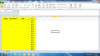
-I have a time sheet and I need to pull data from that sheet and populate Destination Sheet.
-Data which is across rows has to run vertically down a column.
-For example in row 3 in time sheet, project 1 has worked two times in a week, it has two time entry, it has to be repeated two times in destination sheet
-For Example: project 5 has repeated 4 times in a week, so we have to repeat project 5, 4 times in destination sheet
-Sub Project has the same pattern. It has to be repeated vertically down the column based on the count of time entry in front of that
-Please let me know if this is not clear.
-I am sure this has a solution.

I am grateful to you.

GN0001
 

Attachments

  • TimeSheet.xlsx
    20.7 KB · Views: 4
  • Destination.xlsx
    30.4 KB · Views: 3
Narayank,

Yes, that's it, and it is not urgent at all. Please take your time. It was urgent, but it is not any longer.
I appreciate your time that you spend on this,

I also need this to be taken care of without any code if it is possible. Because I don't know VBA.

Thank you for the help and it is not urgent at all.

Please take your time.

GN0001
 
Hi ,

See if this is OK.

Narayan
I think that's it, But let me try first and go to bigger rows and I will let let you know. Also, would you please tell me what you have done, step by step, then I will use evaluate formula to get a hang of it.
Is this an array function?
What are the percentage signs % you have put in the function?
One of the team members tried to help me and I appreciate his/ her help a lot and yours too.

I need to plug in 400 time sheets, If I plug in the second time sheet, will the rows from the second time sheet be added to the destination sheet and will be inserted after row 12 and so on until I finish plugging in the data of all time sheets?

I have not tried it yet though

Thank you very much,
GN0001
 
Last edited:
Hi ,

What we are doing is creating an address of those cells which are not blank in the data range ; BTW , I have defined a named range called Data for the region ='WK_April_04-06'!$C$3:$I$8 , in the TimeSheet.xlsx workbook.

The address is being created using the R1C1 style of addressing ; thus R3C6 will refer to the cell F3 , since column F is column number 6 , while 3 is the row number.

When we pass on an address in this style to the INDIRECT function , we need to use FALSE as the last parameter in the INDIRECT function , since otherwise it will interpret the address in its normal A1 style of addressing.

Thus , if you see the data range , there are values in cells F3 , G3 , E5 , E6 , E7 , E9 ,....

When we use the SMALL(IF(... construct , what we are doing is looking at the first cell in the range that is non-blank , and retrieving its ROW and COLUMN numbers ; for the first cell which is F3 , this will be 3 and 6 ; directly we cannot use these two numbers , so what we do is combine them to form a decimal number such as 3.6 This is done by using the %% symbols , where each % symbol divides the number by 100 ; thus ROW(F3) + COLUMN(F3)% will result in a decimal number 3.06 ; ROW(F3) + COLUMN(F3)%% will result in a decimal number 3.0006

Now , we convert this to text , using the format 0000.0000 , to give us a text string "0003.0006" ; the decimal point is now replaced by the letter C , using the SUBSTITUTE function , so that finally we have an address such as R0003C0006 , which is the same as R3C6.

Passing this to the INDIRECT function results in the function returning us the value which is in cell F3 , which is what we wanted.

Narayan

Hello Narayan,

I hope you are doing fine. Thank you for this interesting function.

I have scanned the formula

Does the Small function returns the smallest number in an array? Or does that return the smallest nth position in an array?

What does this function return?

SMALL({6, 23, 5, 2.3}, 2)

SMALL( array, nth_position )

The example on Tech On the Net Shows:

=SMALL({6, 23, 5, 2.3}, 2) would return 5, however from what I can understand from your formula, it returns the nth position of an object in an array. What is your thought on this?

---------------------------------------------------------

What does step in do in evaluating of a formula? I evaluate the formula step by step? In what way does “Does Step in” help?


When I play with the function to see what it does, or sometimes I double click on the cell to see the formula? I can not get the result back on the cell and instead it gives me the open dialog box. When I cancel the open dialog box, it changes everything to what you can see in this screen shot. The screenshot is below. I hope you see it.

C:\Users\Guity\AppData\Local\Temp\msohtmlclip1\01\clip_image002.jpg


---------------------------------------------------------

Why does Excel ignores 0s in R0003C0006 and represent it as R3C6?

How can we copy and paste an array function to other cells down a column?

So many thanks for your great help. I have learned so many things.

GN0001
 

Attachments

  • upload_2014-4-27_22-26-23.png
    upload_2014-4-27_22-26-23.png
    41.9 KB · Views: 9
Hi ,

The SMALL function does return the nth smallest number in the array ; so if you have a formula such as :

=SMALL({6, 23, 5, 2.3}, 2)

it will return the second smallest number in the array i.e. 5.

In the formula that has been used :

=INDIRECT("TimeSheet.xlsx" & "!" & "R"&SUBSTITUTE(TEXT(SMALL(IF('TimeSheet.xlsx'!Data<>"",ROW('TimeSheet.xlsx'!Data)+COLUMN('TimeSheet.xlsx'!Data)%%),ROW(A1)),"0000.0000"),".","C"),FALSE)

we are first creating an array from the section :

IF('TimeSheet.xlsx'!Data<>"",ROW('TimeSheet.xlsx'!Data)+COLUMN('TimeSheet.xlsx'!Data)%%)

What this array will do is for every cell in the range Data ( which refers to ='WK_April_04-06'!$C$3:$I$8 ) , if the cell is blank , it puts in the value False ( since in the IF statement we have not specified what is to be done if the condition which is being checked is not satisfied ) ; if the cell is not blank , then we are putting in a composite number , which is made up of the ROW number of that cell , and the COLUMN number of that cell as a decimal part. Thus , in your worksheet , the first cell which is non-blank is cell F3 , whose row number is 3 , and column number is 6.

Thus , the first few entries in the array will be :

{FALSE , FALSE , FALSE , 3.0006 , 3.0007 , FALSE , FALSE ;
FALSE , FALSE , FALSE , FALSE , FALSE , FALSE , FALSE ;
FALSE , FALSE , 5.0005 , 5.0006 , 5.0007 , FALSE , FALSE ;
....

Now , when this array is passed through the SMALL function , the FALSE values are ignored , and the first smallest value which is returned will be 3.0006 , the next will be 3.0007 , then 5.0005 and so on.

Using the TEXT function on 3.0006 will make it 0003.0006

Using the SUBSTITUTE function on this will make it 0003C0006

Prefixing this with the letter R makes it R0003C0006

Putting this within the INDIRECT function , returns 8.25 , which is the value to be found in cell F3.

Narayan

Narayan,
Please give me some time to think about it.
Why when I click on the cell to see the formula in the cell, it gives me open dialog box?
Regards,
GN0001
 
Hi ,

The INDIRECT function does not work with closed workbooks ; thus , when your Time Sheet file is not open , all the results in the Destination file will be error values ; only when the Time Sheet file is opened , will the results appear in the Destination file.

Narayan
 
Hi ,

The INDIRECT function does not work with closed workbooks ; thus , when your Time Sheet file is not open , all the results in the Destination file will be error values ; only when the Time Sheet file is opened , will the results appear in the Destination file.

Narayan
Narayan,
I keep both of them open, still, I get what you see in the screen shot when I double click on the cell.
Thanks,
GN0001
 
Hi ,

Since the formulae are array-formulae , clicking on the cell and pressing ENTER will enter the formula as a normal formula , not an array formula ; if you click on the cell , instead of pressing the ENTER key , press the ESC key to exit from EDIT mode. This will leave the array formula intact.

Narayan
Narayan,
Let me try it, Please.
Thanks,:)
GN0001
 
Narayan,
Let me try it, Please.
Thanks,:)
GN0001
Naryan,
I came to work on the function to learn it.
I faced up with this problem:

The destination workbook was not showing any value, while time sheet workbook was open,
A dialog box was being shown up, asking for update
Then the message was: "it is not connecting to server....."
I came back to Chandoo to download the file to my computer again

Do you think what is the problem? I hit ESC, it didn't help. I hit ctrl+Shif+Enter, it didn't help. The function was on the formula bar (when I kept the mouse over the cell, the formula was being showing on the formula bar).

This problem persists. As soon as, a move or anything happens, the array formulas are gone and REF is being shown in hour column.


My second questions is:

If you say :

"The SMALL function does return the nth smallest number in the array ; so if you have a formula such as :

=SMALL({6, 23, 5, 2.3}, 2)

it will return the second smallest number in the array i.e. 5."

Then in this function:

(SMALL(IF('C:\Users\GN0001\Downloads\TimeSheet.xlsx'!Data<>"",ROW('C:\Users\GN0001\Downloads\TimeSheet.xlsx'!Data)+1%%),ROW(A1))

It looks at the first row, gets the row number, then small function has to pick up the smallest number in array data for first row.

The smallest number on the row is 4.25, however your first row brings back 8.25 which a correct number.

Please let me know if this is clear.

Regards,
GN0001
 
Hi ,

In the formula you have posted , i.e.

SMALL(IF('C:\Users\GN0001\Downloads\TimeSheet.xlsx'!Data<>"",ROW('C:\Users\GN0001\Downloads\TimeSheet.xlsx'!Data)+1%%),ROW(A1)

the IF statement does the following :

where ever the range named Data is non-blank , return the corresponding row number + 1%%.

What this does is different from what you have posted ; this does not return the individual numbers in the data range ; instead , it returns the project name , since that is what is there in the first column of every row.

Thus if the formula sees 4.25 or 8.25 or any other non-blank cell in row 1 , it will return the value 1.0001 ; if it sees any non-blank cell in row 2 , it will return the value 2.0001 ; thus , for every non-blank cell in the data range , it will return the project name for that value.

Narayan
Hello Narayan,
You say this formula:

SMALL(IF('C:\Users\GN0001\Downloads\TimeSheet.xlsx'!Data<>"",ROW('C:\Users\GN0001\Downloads\TimeSheet.xlsx'!Data)+1%%)
return the corresponding row number + 1%%.

This is correct, then why do you use Small function? ROW('C:\Users\GN0001\Downloads\TimeSheet.xlsx'!Data)+1%%) brings back 1.0001, and that means first row and first column.

What does Row(A1) do in Small formula on the top?

Thanks,
GN0001
 
Hi ,

Generally speaking , when ever we use the SMALL function , we will use the ROW(A1) as a parameter ; ROW(A1) evaluates to 1 , but when you copy it downwards , the ROW(A1) changes to ROW(A2) , ROW(A3) , ROW(A4) ,... which evaluate to 2 , 3 , 4 ,...

Thus using the ROW(A1) is an easy way of auto-incrementing that parameter.

The same principle holds true when we use the SMALL function with COLUMN(A1) as the parameter ; when we copy this across a row , in the first column where this is used ( whichever column it may be ) , it will evaluate to 1 , and as we copy it across columns , it will change to COLUMN(B1) , COLUMN(C1) ,... which will evaluate to 2 , 3 ,...

Narayan
 
Hi ,

In the formula you have posted , i.e.

SMALL(IF('C:\Users\GN0001\Downloads\TimeSheet.xlsx'!Data<>"",ROW('C:\Users\GN0001\Downloads\TimeSheet.xlsx'!Data)+1%%),ROW(A1)

the IF statement does the following :

where ever the range named Data is non-blank , return the corresponding row number + 1%%.

What this does is different from what you have posted ; this does not return the individual numbers in the data range ; instead , it returns the project name , since that is what is there in the first column of every row.

Thus if the formula sees 4.25 or 8.25 or any other non-blank cell in row 1 , it will return the value 1.0001 ; if it sees any non-blank cell in row 2 , it will return the value 2.0001 ; thus , for every non-blank cell in the data range , it will return the project name for that value.

Narayan

Hello Narayan,

Thank you for your patience with me, I am working on the function in column 1 and Row 8.

I am in Row 8 and I have values in row 8, I get the corresponding row number + 1%%
I understand it returns the project number, since 8.0001 is translated R8C1 (with substitute functions and text functions and ...), then what is the role of small function? If we get the project number by Row number, why do we need small function here? Secondly, If we need small function why role does the result of Row(A10) which evaluates to 10 play in small function?

Does it refer to element/ object/ number/ text that are in 10th position of array data?

Thanks,
GN0001
 
Hi ,

As long as you have questions , I will try my best to answer them.

1. We need the SMALL function because at each stage we are looking at the same array of results ; this array is being created again and again , by the construct :

IF(TimeSheet.xlsx!Data<>"",ROW(TimeSheet.xlsx!Data)+1%%)

What this does is create an array of values ; where ever the corresponding cell in the TimeSheet.xlsx file in the range named Data is non-blank , the array will have the value from that cell ; where the cell is blank , the array will have the value FALSE since the IF statement has no third parameter.

Thus from row 1 through row 11 ( there are 11 non-blank cells in the TimeSheet ), the array will be the same , and it will be as follows :

{FALSE,FALSE,FALSE,3.0001,3.0001,FALSE,FALSE;
FALSE,FALSE,FALSE,FALSE,FALSE,FALSE,FALSE;
FALSE,FALSE,5.0001,5.0001,5.0001,FALSE,5.0001;
FALSE,6.0001,FALSE,FALSE,FALSE,FALSE,FALSE;
FALSE,FALSE,FALSE,FALSE,7.0001,FALSE,FALSE;
FALSE,FALSE,8.0001,8.0001,FALSE,8.0001,FALSE}

From the above , we can see that we need to retrieve the numbers alone as follows :

3.0001
3.0001
5.0001
5.0001
5.0001
5.0001
6.0001
7.0001
8.0001
8.0001
8.0001

To do this , we need to use the SMALL function , which ignores FALSE values , and retrieves only the numbers , one by one.

2. You can simplify the entire formula , since we always want to retrieve the text from column 1 , by changing the formula slightly , but I wanted to keep the structure the same , which is why I went with the 1%% usage. The simplification would be :

=IF(ISERROR($D2),"",INDIRECT("TimeSheet.xlsx" & "!" & "R"&SUBSTITUTE(TEXT(SMALL(IF(TimeSheet.xlsx!Data<>"",ROW(TimeSheet.xlsx!Data)),ROW(A1)),"0000.1"),".","C"),FALSE))

where the 1 is put in as a fixed part of the format , and within the IF statement we take only the ROW.

Narayan

Narayan,
I understood. :awesome: I am going to practice it a lot, may be I become:awesome:
GN0001
 
Back
Top