Stephan
Member
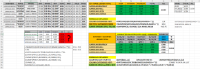
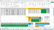
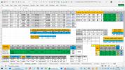
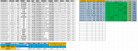
Hello. File attached, see 3rd TAB on right: SUM LEDGER 2 COLUMN
Made LEDGER, of 2 TABLES. 1st Table with SUMIFS of 3 Criteria, however Spill returns Zero so only manual copy & paste edits work.
2nd Table with SUMIFS of 3 Criteria, SPILL returns correctly so sum is 1 cell, so how to do it with ref of 1 SPILL in 2 columns? N2&O2 are N2#
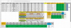
QUESITON 1. How to make Table 1: 3 Criteria SPILL WORK?
Table 2: 3 Criteria SPILL (WORKS)
Table 1: 3 Criteria SPILL (DOESN'T not WORK) Possibly as 1ST 2 COLUMNS (N&O) are 1 SPILL ie N2# is really the spill, but 2nd Column is O2, but O2# gets wrong results.
INDEX: NO wrong
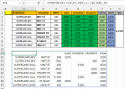
Table 2: 3 Criteria Sum Individal 1st Cell example (WORKS) Without HASH # obviously this SUM works, but not that dynamic as rows will vary depending on data.
QUESTION 2: TABLE FIRST 2 COLUMNS are: BUSINESS & VILLAGE, however I notice 2nd COLUMN is not in AZ order.
How to SORT SPILL: 1st COLUMN AZ, then sort 2nd COLUMN AZ? SORTBY variation? I notice Data was AZ it wouldn't matter, but it is what it is. Hence how to.
Currently the SPILL for the Table 1 COLUMN 1+2 is below. Perhaps another variation of this Formula. I realise can select Col order, but this is either 1st or 2nd?
Google suggested this, but it display RESULTS twice, so that wrong.
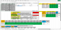
Made LEDGER, of 2 TABLES. 1st Table with SUMIFS of 3 Criteria, however Spill returns Zero so only manual copy & paste edits work.
2nd Table with SUMIFS of 3 Criteria, SPILL returns correctly so sum is 1 cell, so how to do it with ref of 1 SPILL in 2 columns? N2&O2 are N2#
QUESITON 1. How to make Table 1: 3 Criteria SPILL WORK?
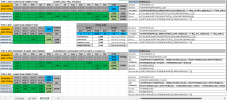
Table 2: 3 Criteria SPILL (WORKS)
=SUMIFS(PRICES,BUSINESS, $N15#, SOLD,">="&QTR_S, SOLD,"<="&QTR_E)
Table 1: 3 Criteria SPILL (DOESN'T not WORK) Possibly as 1ST 2 COLUMNS (N&O) are 1 SPILL ie N2# is really the spill, but 2nd Column is O2, but O2# gets wrong results.
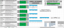
I perceive fault lies with 1st & 2nd COLUMN (N&O) referenced to in SUMSIFS 3 CRITERIA as seperates, N2# & O2# are actually same SPILL in N2#. How to make 2 column spill with 2 seperate Spill refs to work? Perhaps compare lists with ref as 2 different spills that correspond with adjacent COLUMN? If so quite a trick? Hopefully easier solution will present it self! Did investigate INDEX & OFFSET, but numbers are wrong:=SUMIFS(PRICES, BUSINESS, $N2#, VILLAGE,$O2#, MAKES,$P$1#)
INDEX: NO wrong
OFFSET: NO wrong= SUMIFS(PRICES, BUSINESS, $N2#, VILLAGE,INDEX(N2#, , 2), MAKES,$P$1#)
= SUMIFS(PRICES, BUSINESS, $N2#, VILLAGE,OFFSET(N2#, 0,1), MAKES,$P$1#)
Table 2: 3 Criteria Sum Individal 1st Cell example (WORKS) Without HASH # obviously this SUM works, but not that dynamic as rows will vary depending on data.
= SUMIFS(PRICES, BUSINESS, $N2, VILLAGE,$O2, MAKES,$P$1)
QUESTION 2: TABLE FIRST 2 COLUMNS are: BUSINESS & VILLAGE, however I notice 2nd COLUMN is not in AZ order.
How to SORT SPILL: 1st COLUMN AZ, then sort 2nd COLUMN AZ? SORTBY variation? I notice Data was AZ it wouldn't matter, but it is what it is. Hence how to.
Currently the SPILL for the Table 1 COLUMN 1+2 is below. Perhaps another variation of this Formula. I realise can select Col order, but this is either 1st or 2nd?
=SORT(UNIQUE(FILTER(BUSINESS:VILLAGE,BUSINESS<>"")),,,)
Google suggested this, but it display RESULTS twice, so that wrong.
=SORT(UNIQUE(CHOOSE({1,2}, FILTER(DataRange, IncludeCriteria), FILTER(DataRange2, IncludeCriteria))), 1)

Attachments
Last edited:


