Lesliejherrera
New Member
I'm completely new to this, so don't mind my newbie lingo/lack of knowledge.
I have a report that I want to update automatically every week (Mondays) I'll explain everything... consider this a possible challenge. (it is for me)
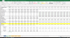
Column A has the information or data that will be going in each row. (I have each cell in columns B through K feeding off info from a tab [FY2016].)
B:3 3/19/2016, C:3 3/26/2016, and so on until K.
Column L (also getting info from a different tab [FY2015]) has K's last year's week.
K:3 5/21/2016
L:3 5/23/2015
I upload information weekly. Every Monday I put in the previous weeks data ending on Saturday.
I need a formula or code...
That can shift the data to the left every Monday so the date will be "fresh." But I don't want to delete columns. I want to have the same amount of columns, only change the info based on the week.
The whole point of the report is to compare the "current" week with last years week.
Column M just subtracts L from K.
If it's not clear, that's mostly because I'm terrible at explaining things.
I would appreciate any help and am open to suggestions..png")
I have a report that I want to update automatically every week (Mondays) I'll explain everything... consider this a possible challenge. (it is for me)
Column A has the information or data that will be going in each row. (I have each cell in columns B through K feeding off info from a tab [FY2016].)
- Date of the week
- Shuttle Hours
- Union Regular Hours
- Union Overtime Hours
- Total Union Hours
- % Overtime Hours
- Avg Hrs Per Run
- Cases Per Stop
- Cases Per Truck
- Stops Per Truck
- CPMH
- Delivery Miles
- Shuttle Miles
- Total Fleet Miles
- Avg Delivery Miles/Trip
- Avg Total Miles/Trip
- Total Runs
- Cases Shipped
- Avg. Piece per Mile
- Total Scheduled Stops
- Shorts
- Miles Efficiency
- Roadnet Miles
B:3 3/19/2016, C:3 3/26/2016, and so on until K.
Column L (also getting info from a different tab [FY2015]) has K's last year's week.
K:3 5/21/2016
L:3 5/23/2015
I upload information weekly. Every Monday I put in the previous weeks data ending on Saturday.
I need a formula or code...
That can shift the data to the left every Monday so the date will be "fresh." But I don't want to delete columns. I want to have the same amount of columns, only change the info based on the week.
The whole point of the report is to compare the "current" week with last years week.
Column M just subtracts L from K.
If it's not clear, that's mostly because I'm terrible at explaining things.
I would appreciate any help and am open to suggestions.